Google Sheets Gradebook Template: Points-Based and Percentage-Based

Here are two ready-to-copy Google Sheets gradebook templates, points-based and percentage-based, plus the steps to build your own from scratch.

Copy a template and start entering scores today, or follow the twelve steps below and build one yourself from scratch. Both work for a classroom teacher and for a homeschooling parent.

The templates

Both templates are ready to copy. Make your own copy, then replace the sample students and assignments with your own.  

Each one has five sample students, working formulas, and letter grades already set up, so you can see what should happen before you put real names in.

Points-based template

Every assignment is worth its points, and the grade is total points earned over total points possible.

A student with 177 of a possible 200 gets 88.5 percent.

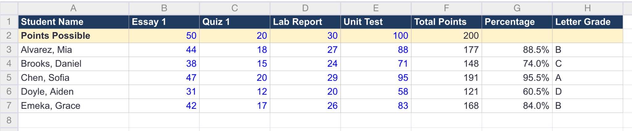
It's the quickest to set up and the easiest for young students and parents to follow, since anyone can see where the marks went.

View or download the points-based Google Sheets gradebook template here.

Percentage-based template

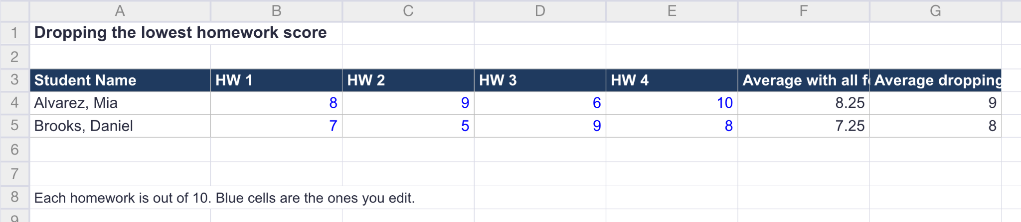
Each category counts for a set share of the final grade. For example, tests 40 percent, homework 30 percent, and participation 30 percent. 

You need a percentage-based gradebook template because a quiz shouldn't count as much as a final exam.

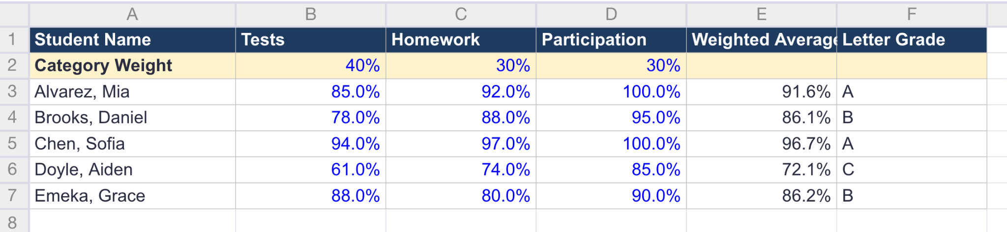
It also has a second tab showing how to drop a student's lowest homework score.

View or download the percentage-based Google Sheets gradebook template here.

Pick points-based if every assignment should count equally, and percentage-based if your categories carry different weights.

You can switch later without starting over, since the student names and scores carry across.

Build your own, step by step

If you would rather build one yourself, here are the twelve steps. The layout they assume is that row 1 holds your headers, row 2 holds the points possible, and your students start on row 3.

Every formula below uses that layout, so if you put your students somewhere else, shift the cell references by the same number of rows. The whole build takes about twenty minutes the first time, and most of that is typing names.

1. Create the sheet

Open Google Sheets, start a blank spreadsheet, and name it with the class and the term, like "Grade 9 English, Fall 2026."

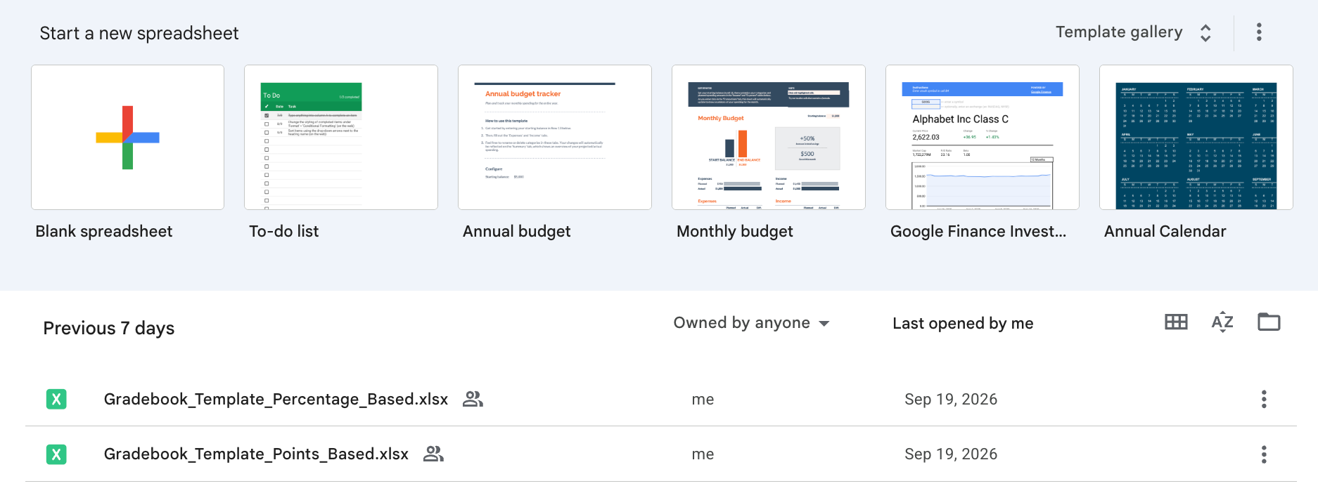
Naming it properly now matters more than it sounds, because by May you'll have four of these open at once and "Untitled spreadsheet" won't tell you which is which.

2. Add your headers

In row 1, put Student Name in column A, then one column for each assignment: Essay 1, Quiz 1, Lab Report, Unit Test.

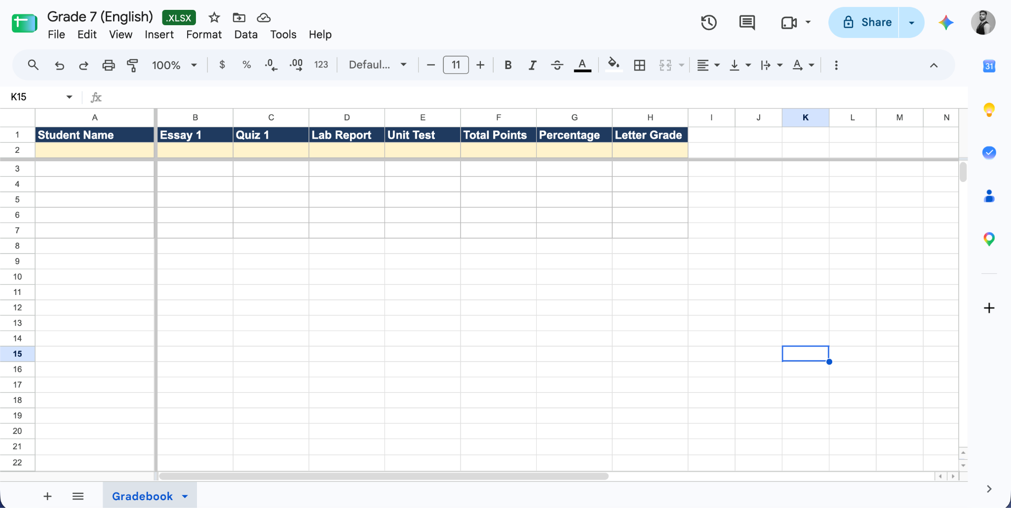
Keep the names short enough to read without widening every column, and add new assignments to the right as the term goes on rather than inserting them in the middle.

3. List your students

Put every student in column A, one per row, alphabetical by last name.

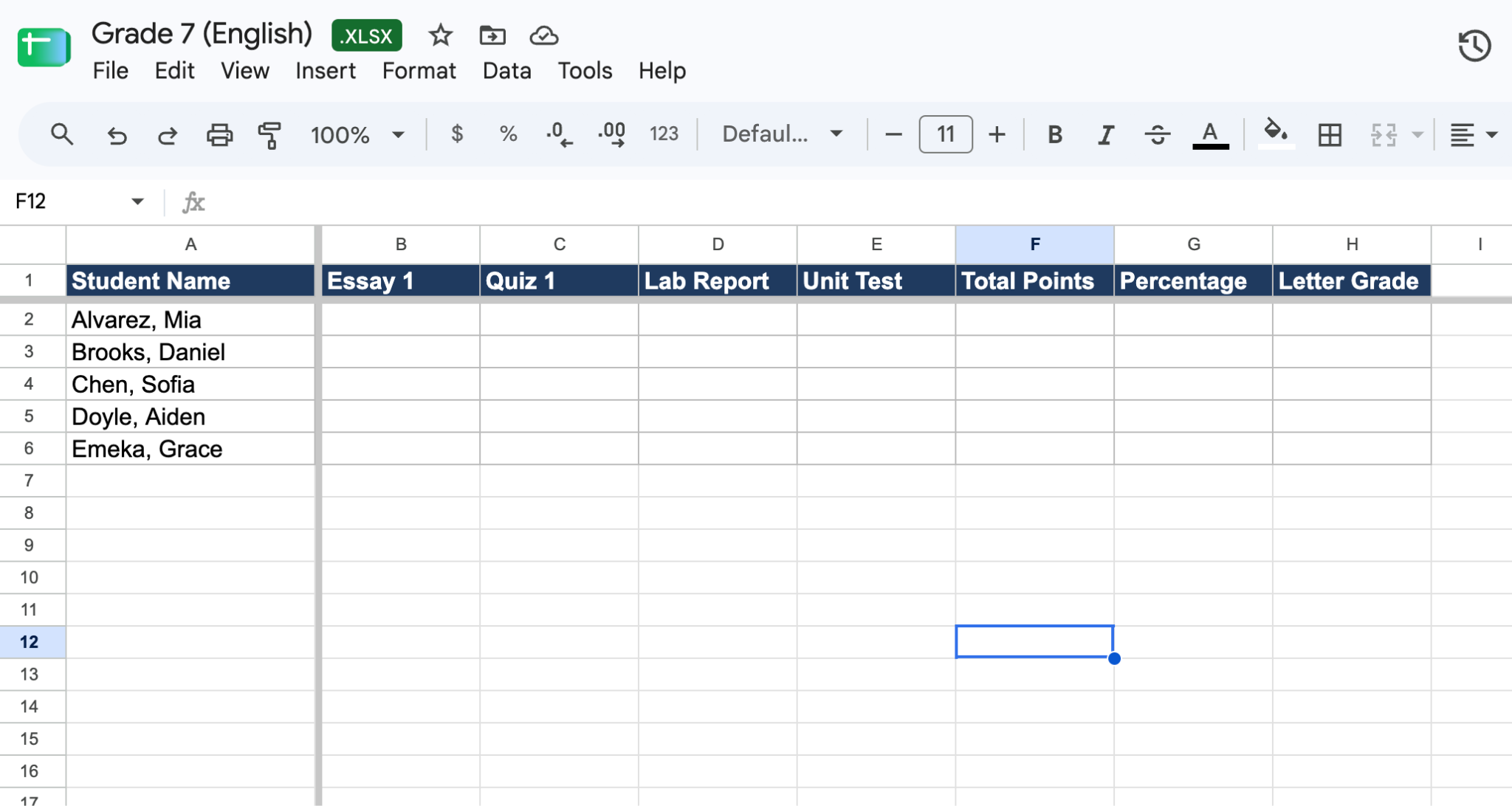
That order matches most class lists and attendance sheets, which saves you hunting when you're entering a stack of marks. If your school uses student ID numbers, add them in column B and shift the assignments one column right.

4. Add a Points Possible row

In row 2, directly under the headers, enter the maximum score for each assignment: 50 for the essay, 20 for the quiz, and so on. 

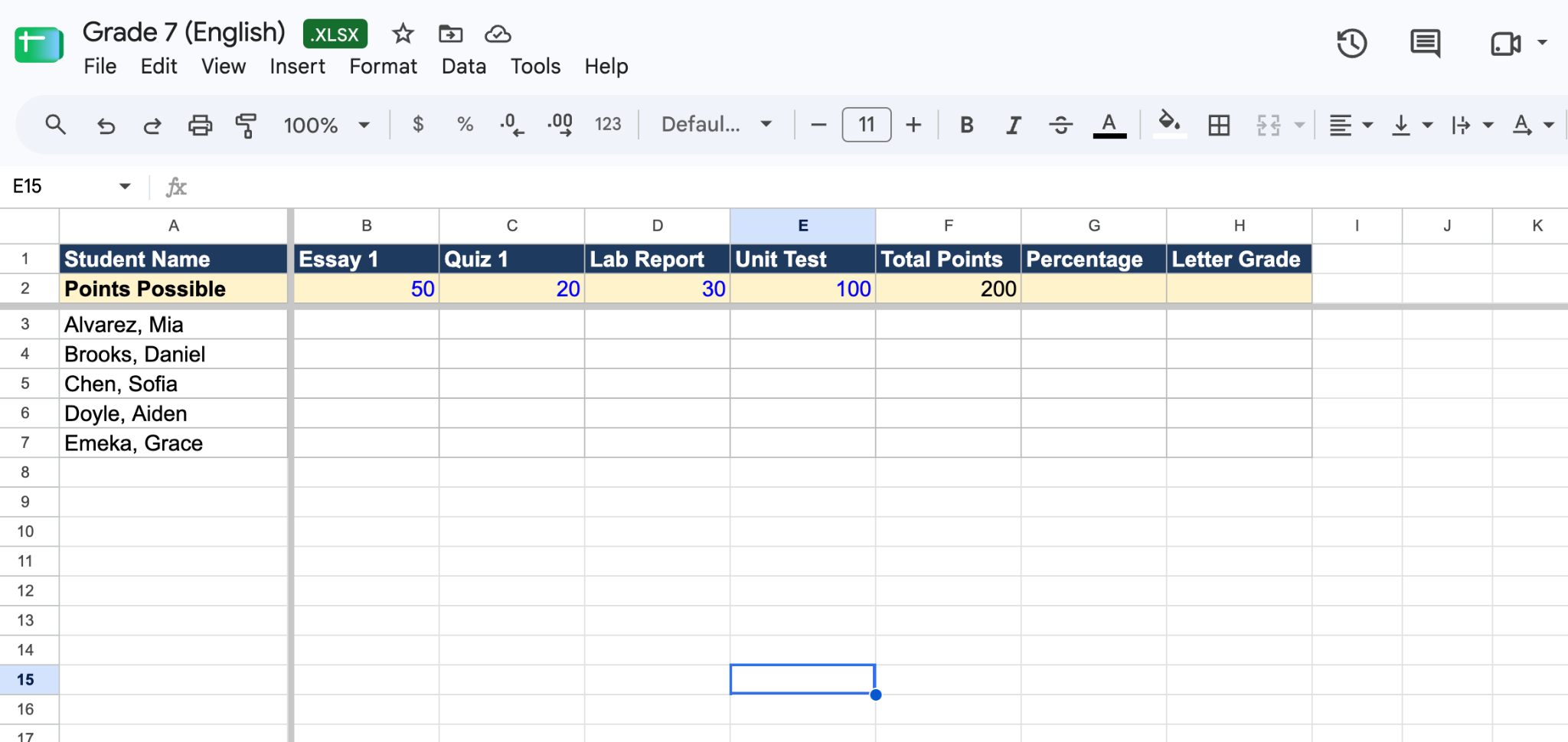
Every percentage on the sheet reads from this row, so it has to be filled in before the formulas will mean anything.

5. Enter scores as work comes in

Type each student's score in the cell where their row meets the assignment column. Leave the cell blank for work you haven't marked yet, and don't type a zero until the deadline has passed.

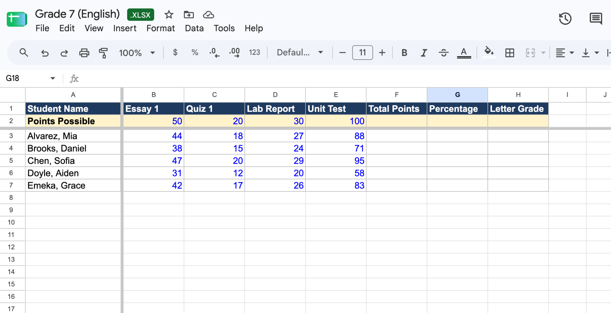
A zero entered early drags a student's average down and then sits there long after the work has been handed in.

6. Add a Total Points column

In the first empty column to the right of your assignments, add the header Total Points, then in the first student's row enter =SUM(B3:E3).

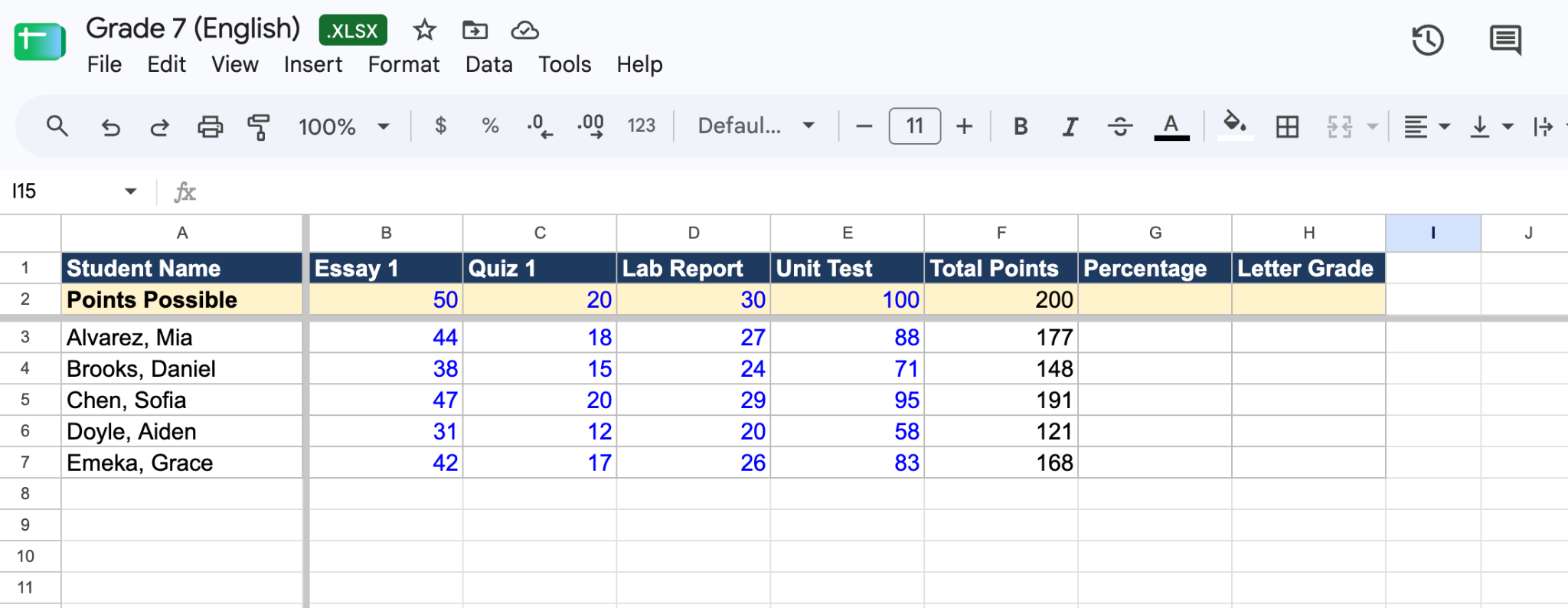
Adjust the range so it covers your assignment columns. Drag the formula down the column, or copy the cell and paste it into the rest of the rows.

7. Add a Percentage column

Next to it, add Percentage and enter =SUM(B3:E3)/SUM($B$2:$E$2), then format the column as a percentage with Format, Number, Percent. The dollar signs lock the formula onto row 2 so it keeps pointing at the points possible as you drag it down.

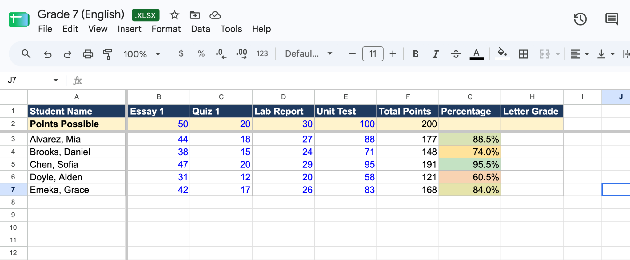
One problem is that this version treats a blank cell as a zero, so if you leave ungraded work blank, use =SUM(B3:E3)/SUMPRODUCT((B3:E3<>"")*$B$2:$E$2) instead, which counts only assignments that have a score.

8. Turn the percentage into a letter

Add a Letter Grade column with =IFS(G3>=0.9,"A",G3>=0.8,"B",G3>=0.7,"C",G3>=0.6,"D",TRUE,"F"), changing G3 to your percentage cell and the cutoffs to your school's scale. 

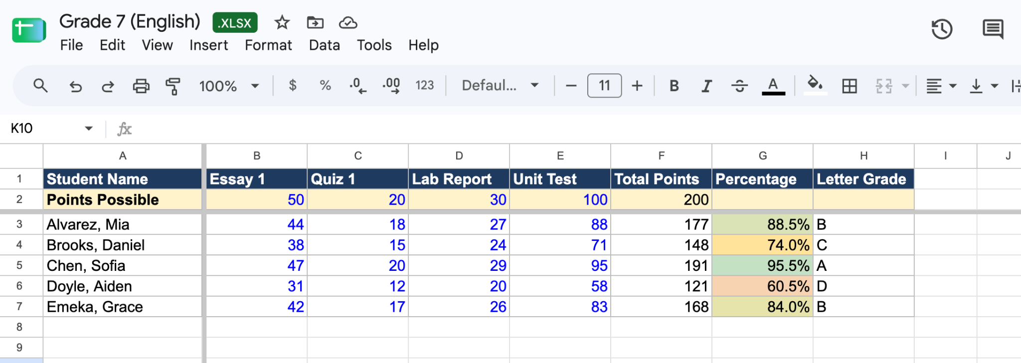
IFS reads the conditions in order and stops at the first true one, so the cutoffs have to run from highest to lowest.

9. Freeze the headers

Click any cell, then go to View, then Freeze, then choose 1 row, and repeat with 1 column. 

Names and assignment headers now stay put while you scroll, which is the difference between entering marks for 32 students confidently and entering one of them on the wrong row.

10. Add conditional formatting

Select the percentage column, then Format, then Conditional formatting, and pick the Color scale tab. 

Low percentages shade one color and high ones another as you type, so a student sliding from 72 to 61 percent shows up while there's still term left to do something about it.

11. Protect the formula columns

Select the Total Points, Percentage, and Letter Grade columns, then go to Data, then Protect sheets and ranges (right-clicking the selection and choosing Protect range gets you to the same place). Set it to show a warning when editing.

One stray paste into a formula column is otherwise enough to wipe a term's calculations without you noticing.

12. Share it carefully

Use the Share button for anyone who should see the whole sheet, like a co-teacher or an administrator.

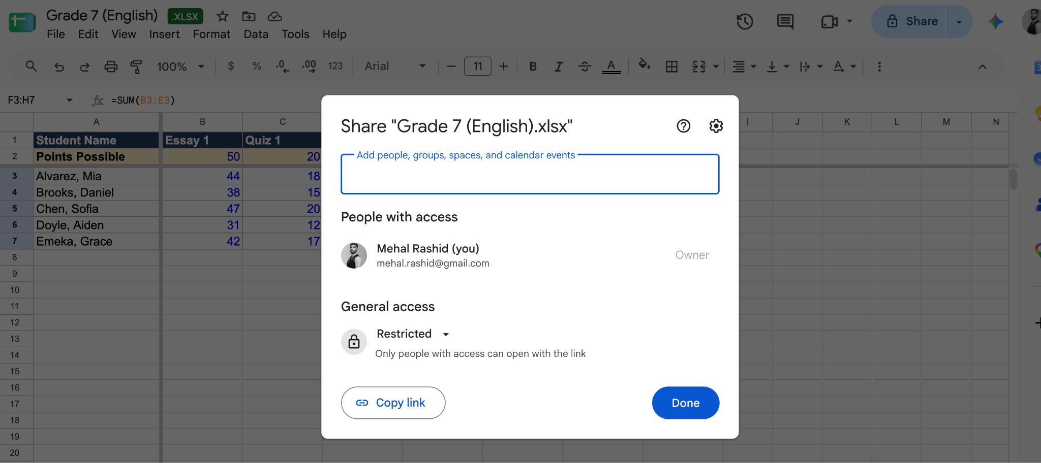
Students and parents should never get the class sheet, since it shows every other student's marks. Send an individual student a screenshot of their own row, or keep a separate sheet per student.

Weighting assignment categories

If assignment categories carry different weights, one formula replaces the simple percentage above. Put each category's weight in row 2 and each student's percentage for that category in their own row.

• Weighted average. With tests at 40 percent, homework at 30 percent, and participation at 30 percent, the formula is =SUMPRODUCT(B3:D3,$B$2:$D$2)/SUM($B$2:$D$2). Take a student who has 85 percent on tests, 92 percent on homework, and 100 percent on participation. SUMPRODUCT multiplies each percentage by its weight and adds the results: 34 plus 27.6 plus 30 gives 91.6, which, divided by the total weight of 100, comes to 91.6 percent, an A on most scales. Notice that the plain average of those three numbers is 92.3 percent, so the weighting does change the letter for students near a boundary.
• Dropping the lowest score. For a homework category where you drop the worst result, use =(SUM(B3:E3)-MIN(B3:E3))/(COUNT(B3:E3)-1). A student with homework scores of 8, 9, 6, and 10 out of 10 averages 8.25, or 82.5 percent. Drop the 6, and the remaining three total 27, divided by 3, that gives 9 out of 10, or 90 percent. Both formulas are already built into the percentage-based template if you'd rather not type them.

Which categories you weight, and whether you drop scores at all, follows from how your school reports grades.

Our guide to types of grading systems covers the main approaches and what each one is trying to show.

For homeschool families

A homeschool gradebook has one column most classroom gradebooks do not need: the subject. A classroom teacher usually keeps one sheet per class. At home, you have one child across six or seven subjects, which is a different shape.

The setup that works best is one spreadsheet per child, with a tab for each subject: Math, Reading, Science, History. Each tab is just the points-based layout from above. 

Adding a summary tab that pulls each subject's percentage gives you a single view for the end of the year, which is what a portfolio review or a state reporting form usually asks for.

Keep it points-based unless you have a reason not to. Weighted categories are best suited for complexity in a class of 30 with four assessment types. 

With one or two learners and a handful of assignments a month, total points over points possible tells you the same thing with less to maintain. Every formula above works unchanged, one tab at a time.

What you need to record varies by state, so it's worth checking your own requirements before you decide how much detail to keep.

Some families need a percentage per subject and nothing more, while others want attendance, hours, and a work sample alongside it, and that decision is easier to make in August than in April.

Where a spreadsheet stops being enough

A spreadsheet records the grade. It does not explain it. The cell holds 82 percent, and nothing in the sheet says why that essay landed there, what the student should fix, or which criteria they actually met.

That gap shows up in three places. There's nowhere to attach feedback to a grade, so the comments live on the document, in an email, or on paper while the number lives in the sheet. 

There's no rubric behind the number, so a B from September and a B from May might mean different things. And everything is manual, so each new term starts with rebuilding columns and re-entering names.

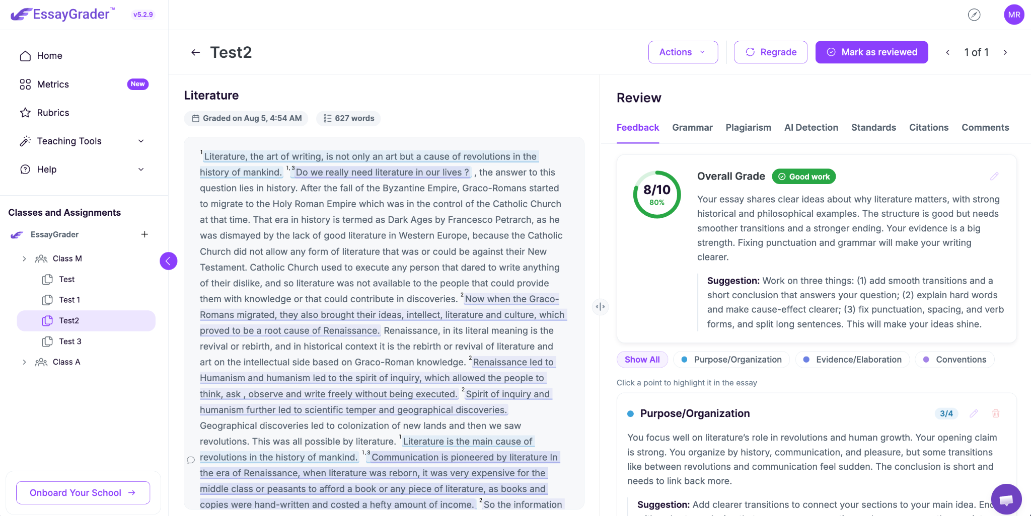
EssayGrader, a rubric-based AI essay grading platform for K-12 and higher-education teachers, closes that gap for written work. It grades essays against the rubric criteria you define and returns the grade with the feedback attached to it, so the record and the reasoning stay together. 

You can browse the rubric library if you'd rather start from an existing writing rubric, and see the full feedback record for what a teacher actually gets back.